Descriptive statistics (dispersion, pt. 2)
Comparing descriptive statistics
Fill in the missing code to compare descriptive statistics for population data at the county level for two states. Before computing statistics though, make predictions:
- Which state has the greater mean?
- Which has the greater median? Which has the greater maximum value?
- Which has the lower minimum value?
- Which has the greater kurtosis and skew?
- Which has the greater standard deviation?
## load packages
library(tidycensus)
library(dplyr)
library(haffutils)
library(e1071)

## load api key here if necessary
census_api_key("add your key here")

## get population data from the census

## get state fips as its own variable

## filter by state (get two states)

## density plots

## central tendency

## shape

## dispersion
Compare two other states!
Use one of the following variables and compare again:
B15003_022(but you should probably normalize byB01003_001!)B07013_002(this one should also be normalized byB01003_001!)
Additionally, create maps of the data using
tmap
Comparing standard deviations
library(truncnorm)
library(dplyr)
library(reshape2)
library(ggformula)

n <- 1e4

x1 <- runif(n, min = 1, max = 5)
x2 <- c(rtruncnorm(n/2, a=1, b=5, mean=2, sd=.5),
        rtruncnorm(n/2, a=1, b=5, mean=4, sd=.5))

df <- data.frame(x1 = x1, x2 = x2) %>%
  melt()

gf_histogram(~ value | variable, data = df, fill = ~ variable)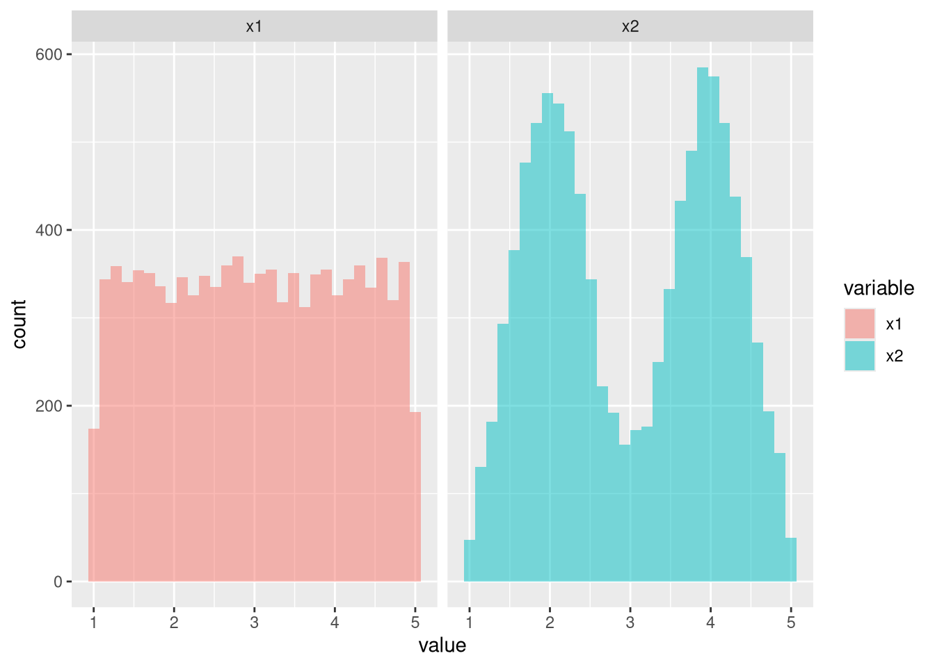
gf_density(~ value, data = df, fill = ~ variable)
## which has the greater standard deviation?