Exam 4 overview
Exam structure
- 18 multiple choice (1 pt. each)
- 4 TRUE/FALSE (0.5 pt. each)
- 5 numerical answer (1 pt. each)
Conceptual question topics
Correlation
- Be able to differentiate between assumptions for Pearson’s r and Spearman’s \(\rho\).
- Be able to look at a correlogram and note which relationships are:
- Significant or insignificant
- Strong or weak
- Positive or negative
Regression
- Be able to explain the various assumptions of OLS
- Given a regression equation, be able to state how y changes with x (in terms of number of units)
- Given a regression equation, be able to explain the meaning of the y-intercept.
- Be able to explain the modifiable areal units problem (MAUP) and be familiar with examples of how it relates to quantitative methods
- Know the ways in which performance is measured in a regression model:
- Coefficient of determination
- F-test and p-value
- AIC
- Given a regression result, be able to explain which variables are significant at a given p-value.
Spatial autocorrelation
- Know the difference between positive and negative spatial autocorrelation
- Given a map of local spatial autocorrelation results, be able to explain
where the following are present:
- Significant HIGH-HIGH spatial autocorrelation
- Significant LOW-LOW spatial autocorrelation
- Insignificant spatial autocorrelation
- Be able to explain the various neighboring schemes used in computing
spatial autocorrelation and how many neighbors each would produce given an
example:
- Queen’s, rook’s, and bishop’s contiguity
- knn
- Distance band
- Given a set of results for Moran’s I, be able to explain at which bandwidths there is significant spatial autocorrelation.
Computation questions
Be prepared to make the following computations in R:
- Correlation analysis using the
corfunction and the appropriatemethod. - A correlation test using the
cor.testfunction and the appropriatemethod. - Regression analysis using the
lmfunction using appropriate dependent and independent variables. - A calculation of variance inflation factor (VIF) using the
viffunction from the car package.
These computations will be conducted on the datasets below. Feel free to start exploring them before the exam!
swissOrchardSprayscars(note this is different frommtcars!)
Practice questions
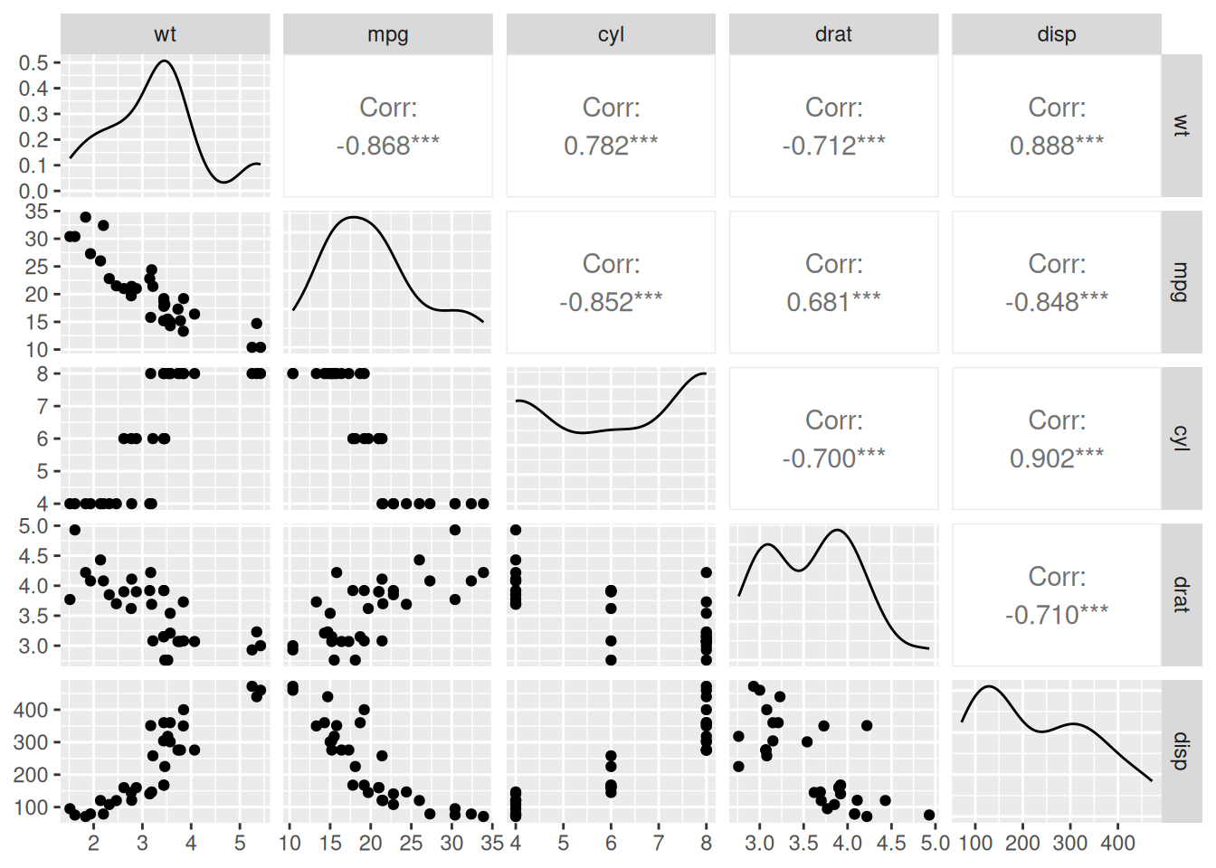
Given the following correlogram, state the following:
- The strongest relationship
- The weakest relationship
- The shape of the variable
drat - The nature of the relationship (strong/weak/positive/negative) between
mpganddisp
Answer the questions associated with the following regression results:
- Which variables are significant at p < 0.10 in the model?
- What percentage of the DV is explained by the model?
- What is the direction of influence for the variables
gearandcylon the DV? - Is the model strong or weak?
##
## Call:
## lm(formula = mpg ~ wt + disp + cyl + drat + gear + carb, data = mtcars)
##
## Residuals:
##     Min      1Q  Median      3Q     Max
## -3.8332 -1.5559 -0.2125  1.3036  5.5991
##
## Coefficients:
##              Estimate Std. Error t value Pr(>|t|)
## (Intercept) 29.376002  11.069779   2.654   0.0136 *
## wt          -2.436813   1.403502  -1.736   0.0948 .
## disp        -0.002092   0.013411  -0.156   0.8773
## cyl         -0.860657   0.865913  -0.994   0.3298
## drat         1.104622   1.578304   0.700   0.4905
## gear         0.813645   1.354587   0.601   0.5535
## carb        -0.928269   0.634316  -1.463   0.1558
## ---
## Signif. codes:  0 '***' 0.001 '**' 0.01 '*' 0.05 '.' 0.1 ' ' 1
##
## Residual standard error: 2.611 on 25 degrees of freedom
## Multiple R-squared:  0.8487,	Adjusted R-squared:  0.8124
## F-statistic: 23.37 on 6 and 25 DF,  p-value: 4.056e-09
Answer the questions below given the following Moran’s I results:
- At which bandwidths are results significant at p < 0.05?
- Would you say there is significant spatial autocorrelation in this dataset?
## Reading layer `wi_hazards' from data source
##   `https://gitlab.com/mhaffner/data/-/raw/master/wi_hazards.geojson'
##   using driver `GeoJSON'
## Simple feature collection with 72 features and 16 fields
## Geometry type: MULTIPOLYGON
## Dimension:     XY
## Bounding box:  xmin: -92.88811 ymin: 42.49198 xmax: -86.80542 ymax: 47.08062
## Geodetic CRS:  NAD83
## neighbors morans_i variance p.value
## 1 3 0.27272946 0.019071164 0.0189062555
## 2 6 0.17419275 0.010496077 0.0330502777
## 3 9 0.17134996 0.007075910 0.0137465239
## 4 12 0.10285532 0.005377042 0.0553848442
## 5 15 0.12067017 0.004210056 0.0189088584
## 6 18 0.09224795 0.003453924 0.0352025700
## 7 21 0.10947707 0.002916663 0.0110711746
## 8 24 0.14712254 0.002516736 0.0006558609Given the following regression equation, a positive change in one unit of \(x_{3}\) would result in a change of how many units of \(y\)?
\(Y = -13.57 + 27.03 x_1 - 0.04 x_2 - 14.14 x_3\)
Answer the questions below given the following Moran’s I results:
- At which bandwidths are results significant at p < 0.05?
- At which bandwidth is there the most significant Moran’s I results?
- Would you say there is significant spatial autocorrelation in this dataset?
## neighbors morans_i variance p.value
## 1 2 0.0009689922 0.010172580 0.4406772
## 2 4 -0.0675651868 0.005595502 0.7626809
## 3 6 -0.0561486963 0.003768838 0.7533869
## 4 8 -0.0814570120 0.002864538 0.8959480
## 5 10 -0.0767146129 0.002243023 0.9069843
## 6 12 -0.0271975455 0.001841091 0.6200487
## 7 14 -0.0250369521 0.001554033 0.6094290
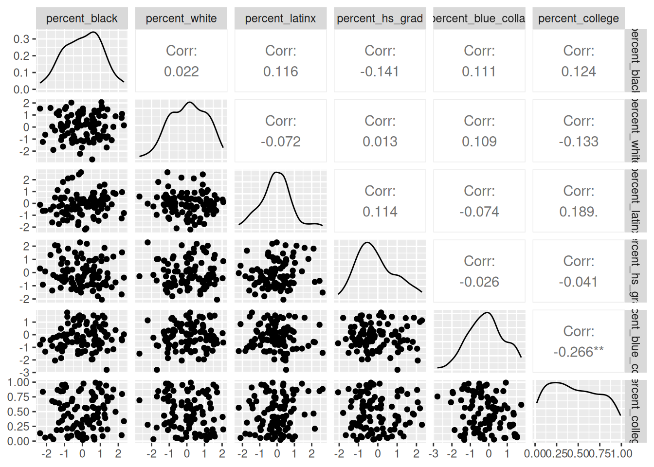
## 8 16 -0.0319312309 0.001341049 0.6869930Given the following correlogram, answer the questions below.
- What is the strength and direction of the relationship between
percent_blackandpercent_latinx? - What is the correlation coefficient of the relationship between
percent_hs_gradandpercent_blue_collar? - Which variable pairs are significantly correlated?
- Would the assumptions for Pearson’s r between
percent_collegeand another variable hold? Why or why not?
- What is the strength and direction of the relationship between
Given the following regression model output, answer the questions below.
- Which variable has the strongest effect on the dependent variable?
- Which variables are significant at p < 0.01?
- A positive change in 10 units of
percent_whitewould have an effect on the dependent variable in how many units? - Is the model significant?
- How would you assess the assumption of normality of residuals?
- How would you assess the assumption of Independence if these were spatial data?
##
## Call:
## lm(formula = percent_college ~ percent_black + percent_white +
## percent_latinx + percent_hs_grad + percent_blue_collar)
##
## Residuals:
## Min 1Q Median 3Q Max
## -0.53518 -0.21972 -0.02336 0.22737 0.61165
##
## Coefficients:
## Estimate Std. Error t value Pr(>|t|)
## (Intercept) 0.45489 0.02864 15.881 < 2e-16 ***
## percent_black 0.03679 0.02781 1.323 0.18913
## percent_white -0.02736 0.02752 -0.994 0.32276
## percent_latinx 0.04790 0.03083 1.554 0.12358
## percent_hs_grad -0.01342 0.02907 -0.462 0.64538
## percent_blue_collar -0.07976 0.03006 -2.654 0.00935 **
## ---
## Signif. codes: 0 '***' 0.001 '**' 0.01 '*' 0.05 '.' 0.1 ' ' 1
##
## Residual standard error: 0.2798 on 94 degrees of freedom
## Multiple R-squared: 0.1287, Adjusted R-squared: 0.08237
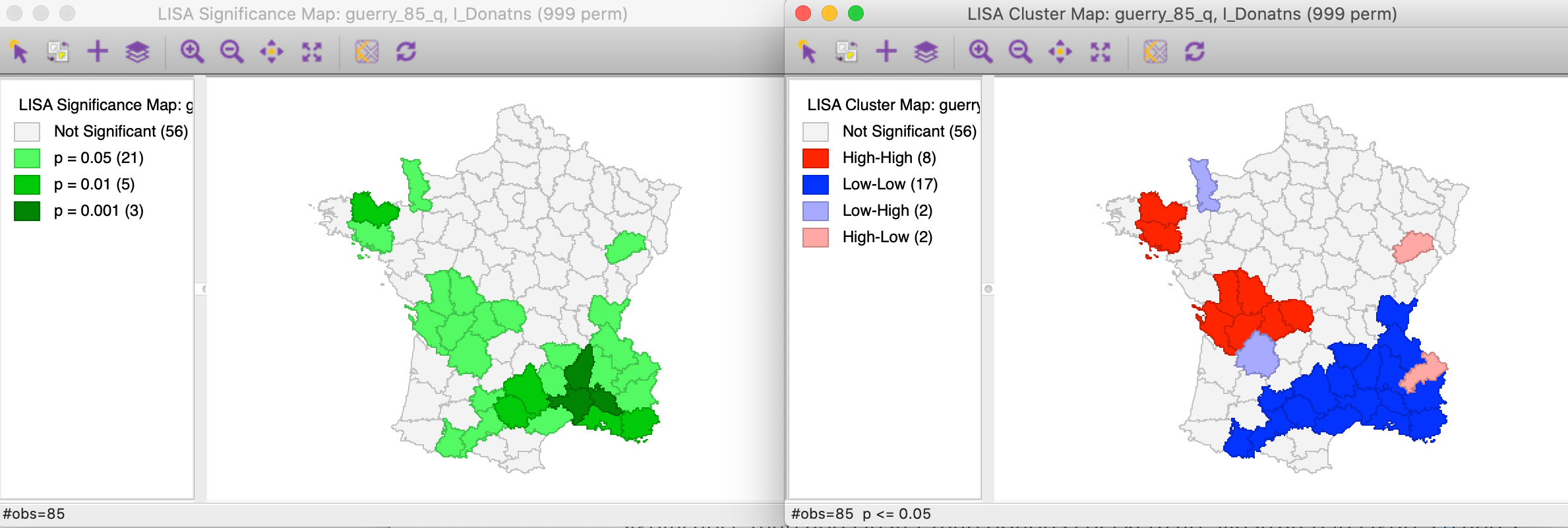
## F-statistic: 2.777 on 5 and 94 DF, p-value: 0.02197Given the following Local Moran’s I result, answer the following questions.
- Does the dataset exhibit more positive or negative spatial autocorrelation? How can you tell?
- Where is there the most significant spatial local autocorrelation?
- What is the nature of local spatial autocorrelation in the northern most zone?
Using the built-in R dataset
USArrests, conduct a correlation test with the variablesMurderandUrbanPop. Answer the following questions:- Which variable should be
yand which should bex? - What is the appropriate
methodto use? - What is the correlation coefficient?
- What is the p-value?
- Which variable should be
Using the dataset
Bostonfrom theMASSpackage, conduct a regression analysis withcrimas the dependent variable and the variablesrm,chas,indus,zn,medv, andnox.- What is the p-value of the model?
- What is the most significant variable in the model?
- What is the coefficient of determination?
- What is the direction of influence for the variable
chas? - What is the direction of influence for the variable
medv? - Which variables possess significant multicollinearity (if any)?
- Which variables are not significant in the model?
- Are the residuals normally distributed?